Chapter 7 Factorial experiments
In this section, we consider experiments where the treatment structure involves multiple experimental factors.
7.1 Combining factors: Crossed vs. nested designs
Experimental factors can be combined in two different ways. The distinction is illustrated by the following two experiments.
Experiment 1. (A hypothetical experiment based on example 15.8 in Ott & Longnecker):
A citrus orchard contains 3 different varieties of citrus trees. Eight trees of each variety are randomly selected from the orchard. Four different pesticides are randomly assigned to two trees of each variety and applied according to recommended levels. The same four pesticides are used for each variety. Yields of fruit (in bushels per tree) are recorded at the end of the growing season.
Experiment 2. A study is conducted to investigate the effect of pest management practices on cotton in the central valley of California. 14 ranches are available for study. Each of the 14 ranches is managed by one consultant.
In both experiments, there are two experimental factors—variety and pesticide in experiment 1, and consultant and ranch in experiment 2. Each unique combination of factors forms a separate treatment combination. In experiment 1, the treatment combinations are formed by crossing the two experimental factors. That is to say, every level of the first factor (variety) is combined with every level of the second factor (pesticide). This is an example of a factorial or crossed design. In experiment 2, each level of one factor (ranch) is only combined with one single level of the other factor (consultant). This is an example of a hierarchical design, and we would say that ranch is nested within the consultant.
Experiments with more than two factors can give rise to designs that involve aspects of both crossed and nested designs. For example, if we three factors—call them factors “A”, “B”, and “C”—we might cross factors A and B and then nest factor C within the A*B cross.
The remainder of this chapter concerns factorial designs. We will begin by studying a two-factor cross. Most of the ideas involved in analyzing factorial designs can be mastered by studying a two-factor cross. We will also study a three-factor design to see how ideas from two-factor designs extend to experiments with more than two factors.
The analysis of factorial designs makes heavy use of the idea of contrasts, so make sure you understand that material well.
7.2 Two-factor ANOVA
In a two-factor design, the two factors can be generically labeled as factors “A” and “B”. The scientific questions of most interest in a two-factor design are:
Does the average response differ among the levels of factor A, and if so, how?
Does the average response differ among the levels of factor B, and if so, how?
Do the differences among the levels of factor A depend on the level of factor B, and vice versa? If so, how? That is to say, is there evidence of an interaction between the two factors?
Example: Oleoresin collected from pine trees. Oehlert (problem 8.5) reports the following data. Low and Bin Mohd. Ali (1985) studied the collection of pine oleoresin by tapping the trunks of pine trees. Tapping involves cutting a hole in the tree trunk and collecting resin that seeps out. This experiment compared four shapes of holes (circle, diagonal, check, or rectangle) and the effect of adding acid (added vs. control) in collecting resin. Twenty-four pine trees were selected from a plantation and were randomly assigned to each of the 8 possible combinations of hole shape and acid. The response is total grams of resin collected from the hole. The data that we will work with are not the actual data but are instead a hypothetical data set for the same design. This is a balanced, replicated 4 \(\times\) 2 factorial experiment with treatment combinations assigned in a CRD.
7.2.1 Interaction plots
For a two-way layout, it is often convenient to visualize the differences among the treatment means with an interaction plot. (Others call these profile plots.) To construct an interaction plot, write the levels of one factor along the horizontal axis, and use the vertical axis to denote the response. Draw lines on the plot for each level of the other experimental factor. Here is an interaction plot for the oleoresin data: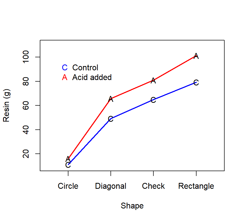
Figure 7.1: Interaction plot for the pine resin data
7.2.2 Getting organized: Notation and bookkeeping
Organization is everything in the analysis of factorial experiments. Organize, organize, organize! To aid in organization, the analysis of factorial designs involves some fairly heavy notation. It’s easy to get lost in the notation. Remember that the notation is not the point. The notation is merely a bookkeeping device for keeping ourselves organized.
Here is some notation that we will use for two-factor experiments:
\(a\): number of levels of factor “A” (for the resin data, we’ll set “acid” as this factor, so \(a = 2\).)
\(b\): number of levels of factor “B” (for the resin data, we’ll set “shape” as this factor, so \(b = 4\).)
\(i = 1, 2, \ldots, a\): an index to distinguish the different levels of factor A (in the resin data, \(i = 1\) for the control, \(i = 2\) for adding acid)
\(j = 1, 2, \ldots, b\): an index to distinguish the different levels of factor B (for the resin data, \(j = 1\) for circles, \(j = 2\) for diagonal incisions, \(j=3\) for checkmark incisions, and \(j=4\) for rectangular incisions)
\(n_{ij}\): sample size for the combination of level \(i\) of factor A and level \(j\) of factor B (in a balanced design, sometimes this gets replaced by \(n\)).
\(k = 1, 2, \ldots, n_{ij}\): an index to distinguish the different replicates within each treatment combination
\(y_{ijk}\): \(k\)th replicate from the combination of level \(i\) of factor A and level \(j\) of factor B.
\(n_T =\sum _{i=1}^{a}\sum _{j=1}^{b}n_{ij}\) : total sample size
\(\bar{y}_{ij+} =\dfrac{\sum _{k=1}^{n_{ij}} y_{ijk}}{n_{ij}}\): sample mean for the combination of level \(i\) of factor A and level \(j\) of factor B
\(\mu_{ij}\) : unknown population mean for the combination of level \(i\) of factor A and level \(j\) of factor B. Sometimes called a “cell mean” because we might think of each treatment combination as corresponding to a “cell” in a table in which each factor corresponds to one of the table’s dimensions.
A marginal mean is the average of all the cell means associated with one level of one factor, averaged over all the levels of the other factor(s). For example, in the resin data, the marginal mean associated with the control (no-acid-added) treatment is \[ \bar{\mu}_{1+} = \dfrac{\mu_{11} + \mu_{12} + \mu_{13} + \mu_{14}}{4}. \] Here, we’ve used a plus (+) subscript to indicate that we are summing over the levels of an index. The marginal mean for the acid addition treatment, \(\bar{\mu}_{2+}\), is defined similarly.
The marginal mean associated with the circular incisions is \[ \bar{\mu}_{+1} = \dfrac{\mu_{11} + \mu_{21}}{2}. \] The marginal means for the other three incision shapes are defined similarly.
7.2.3 ANOVA \(F\)-tests
If all we understood was how to analyze data from a one-way layout, we could conceivably analyze the \(a \times b\) factorial cross using a one-factor ANOVA with \(a \times b\) different treatment groups. This analysis would be unsatisfying, however, because it fails to capitalize on the additional structure provided by the factorial arrangement of the experiment treatments.
The two-factor ANOVA partitions the \(ab-1\) free differences among the \(ab\) treatment means into three contrasts: a contrast of the \(a\) marginal means for factor \(A\) (itself involving \(a-1\) free differences), a contrast of the \(b\) marginal means for factor \(B\) (requiring \(b-1\) free differences), and a contrast that captures the interaction between the two factors (requiring the remaining \((a-1)(b-1)\) free differences. In this way, the two-factor ANOVA goes beyond merely testing if the \(ab\) treatment means differ, and instead tests if the treatment means differ in specific ways suggested by the factorial design.| ANOVA contrast | df |
|---|---|
| Factor A marginal means | \(a-1\) |
| Factor B marginal means | \(b-1\) |
| A*B interaction | \((a-1)(b-1)\) |
In the usual way, testing each of these contrasts entails computing a sum-of-squares associated with each, standardizing that sum-of-squares by its associated df to generate a mean-square, and then comparing the mean-square for the contrast to the MSE to generate an \(F\)-statistic.
When the data are balanced, the ANOVA contrasts are orthogonal, and so the sum-of-squares associated with the three contrasts sum to give the sum-of-squares for the groups, that is, \[ SS_{Groups} = SS[A] + SS[B] + SS[AB]. \] When the data are not balanced, this formula does not hold, but that doesn’t hinder our analysis.
As with one-factor ANOVA, the two-factor ANOVA provides an entry point into the analysis. The ANOVA itself is rarely enough to fully characterize the interesting patterns in the data. To fully analyze the data, the two-factor ANOVA should be followed by customized contrasts of the cell means, multiple comparisons procedures, etc., as we did in one-factor ANOVA.
Before proceeding, let’s analyze the contrasts in the two-factor ANOVA in more detail.
7.2.3.1 Comparisons of marginal means
The two-factor ANOVA provides \(F\)-tests to test for differences among the marginal means of each factor. In the resin example, one \(F\)-test compares the marginal means for control and acid-addition treatments: \[ H_0: \bar{\mu}_{1+} =\bar{\mu}_{2+}. \] A second \(F\)-test tests the null hypothesis that there is no difference between the marginal means for the four shapes: \[ H_0: \bar{\mu}_{+1} = \bar{\mu}_{+2} = \bar{\mu}_{+3} = \bar{\mu}_{+4}. \]
While it may not be immediately obvious, notice that each of these null hypotheses corresponds to a (possibly complex) contrast of the cell means. For example, our test for a difference between the marginal means for the acid-addition treatment can be re-expressed as the (simple) contrast \[ \begin{align} \theta & = \bar{\mu}_{1+} -\bar{\mu}_{2+} \\ & = \dfrac{1}{4}\mu_{11} + \dfrac{1}{4}\mu_{12} + \dfrac{1}{4}\mu_{13} + \dfrac{1}{4}\mu_{14} - \dfrac{1}{4}\mu_{21} - \dfrac{1}{4}\mu_{22} - \dfrac{1}{4}\mu_{23} - \dfrac{1}{4}\mu_{24}. \end{align} \] On the other hand the test for the equality of the four marginal means for the shape treatment is a complex contrast consisting of three linearly independent simple contrasts. One such complex contrast is \[ \begin{align} \theta_1 & = \bar{\mu}_{+1} -\bar{\mu}_{+2} \\ & = \dfrac{1}{2}\mu_{11} + \dfrac{1}{2}\mu_{21} - \dfrac{1}{2}\mu_{12} - \dfrac{1}{2}\mu_{22} \\ \theta_2 & = \bar{\mu}_{+1} -\bar{\mu}_{+3} \\ & = \dfrac{1}{2}\mu_{11} + \dfrac{1}{2}\mu_{21} - \dfrac{1}{2}\mu_{13} - \dfrac{1}{2}\mu_{23} \\ \theta_3 & = \bar{\mu}_{+1} -\bar{\mu}_{+4} \\ & = \dfrac{1}{2}\mu_{11} + \dfrac{1}{2}\mu_{21} - \dfrac{1}{2}\mu_{14} - \dfrac{1}{2}\mu_{24}. \end{align} \]
We will sometimes refer to comparisons of marginal means as the main-effects comparisons associated with a particular factor.
7.2.3.2 Interaction
To think through the interaction, it is helpful to have a bit more terminology at our disposal. We define the simple effect of a factor as the comparisons among the levels of one factor within the level(s) of the other factor(s). For example, in the resin experiment, the simple effect of adding acid to circular incisions is the comparison between circular incisions with acid added vs. circular incisions without acid added. In our notation, this corresponds to the difference
\[
\theta_{\mbox{acid:circle}} = \mu_{21} - \mu_{11}.
\]
Note that this simple-effect comparison is a simple contrast of the cell means. Similarly, we can define the simple effect of acid addition for diagonal incisions as the comparison between diagonal incisions with acid added vs. diagonal incisions without acid added.
\[
\theta_{\mbox{acid:diagonal}} = \mu_{22} - \mu_{12}.
\]
The simple effect of adding acid to checkmark (\(j=3\)) and rectangular (\(j=4\)) incisions can be defined similarly.
An interaction is a comparison of simple effects. In the resin data, the ANOVA \(F\)-test of the interaction corresponds to a test of \[ H_0: \theta_{\mbox{acid:circle}} = \theta_{\mbox{acid:diagonal}} = \theta_{\mbox{acid:checkmark}} = \theta_{\mbox{acid:rectangle}} \] or \[ H_0: \mu_{21} - \mu_{11} = \mu_{22} - \mu_{12} = \mu_{23} - \mu_{13} = \mu_{24} - \mu_{14}. \] This is also a complex contrast. In the case of the resin data, it is a complex contrast that consists of three linearly independent simple contrasts.
Just as with regression, interactions go both ways: if the effect of adding acid differs among the shapes, then the differences among the shapes must also depend on whether acid was added or not.
The interaction plots in Figure 7.1 are helpful for visualizing what is meant by an interaction. The simple effect of adding acid corresponds to the blue-vs-red comparison for a particular shape. The simple effect of shape corresponds to the left-vs-right comparison for one acid treatment or the other. The interaction asks if these simple effects of adding acid are the same for the different shapes, or, conversely, if the simple effects of shape are the same regardless of whether acid was added.
Notice also that we can also define the main-effects comparisons as the averages of the simple effects. For example, the difference between the marginal means of the acid-addition treatment is the average of the simple effects for the acid addition treatment, averaged across shapes. With this recognition comes a crucial point: If the interaction is significant, then we need to be careful about analyzing the main effects, because the main effects are averaging over simple effects that differ. Thus, the usual guidance for breaking down a two-factor ANOVA table is to inspect the interaction first. If the interaction is not significant, proceed to analyze main effects of each factor. If the interaction is significant, then analyze simple effects, and interpret the main-effects comparison cautiously.
7.2.3.3 Back to the resin data
Let’s see how this plays out with the pine resin data. We’ll let the computer calculate the various SS that comprise the ANOVA table for us. For the oleoresin data, we obtain| source | df | SS |
|---|---|---|
| Shape | 3 | 19407 |
| Acid | 1 | 1305 |
| Shape*Acid | 3 | 237 |
| Error | 16 | 721 |
| Total | 23 | 21672 |
| source | df | SS | MS | \(F\) | \(p\) |
|---|---|---|---|---|---|
| Shape | 3 | 19407 | 6469 | 143.5 | <0.0001 |
| Acid | 1 | 1305 | 1305 | 29 | <0.0001 |
| Shape*Acid | 3 | 237 | 79.2 | 1.76 | 0.1961 |
| Error | 16 | 721 | 45.1 | ||
| Total | 23 | 21672 |
Thus, this two-factor ANOVA shows that there is no statistical evidence of an interaction (\(F_{3, 16} = 1.76\), \(p = 0.20\)). Because the interaction is not significant, it makes sense to analyze main effects. There is very strong evidence of a main effect of shape (\(F_{3, 16} = 143.5\), \(p < 0.0001\)) and a main effect of the acid treatment (\(F_{1, 16}\) = 29.0, \(p < 0.0001\)). Because the main effects are significant (and the interaction is not significant), then we can use linear contrasts and multiple comparisons procedures to analyze the marginal means of both factors just as we would in a one-factor layout. For example, we could use a MEANS statement to compare treatment means using multiple comparisons. Here is code for a Tukey’s HSD comparison of the marginal means for the hole shapes:
proc glm data=resin;
  class shape acid;
  model resin = shape acid shape*acid;
  means shape / tukey;
run;

Tukey's Studentized Range (HSD) Test for resin
Means with the same letter are not significantly different.

Tukey
Grouping          Mean      N    shape
A               90.333      6    rectangl
B               73.000      6    check
C               57.500      6    diagonal
D               13.667      6    circular
Thus, all of the shapes are significantly different from one another.
Just as with a one-factor ANOVA, the sums-of-squares in a balanced two-factor ANOVA can be computed using computing formulas that involve nothing more than addition, subtraction, multiplication, and division. These computing formulas were more important in the days before desktop computing. While there may be some small historical value to seeing how this worked, we won’t be computing these quantities by hand today. The formulas follow for completeness, but don’t feel compelled to study them.
The computing formulas begin with the usual one-factor SS decomposition: \[\begin{eqnarray*} \mbox{Total variation: } SS_{Total} & = & \sum_{i=1}^{a}\sum_{j=1}^{b}\sum_{k=1}^{n_{ij} }\left(y_{ijk} -\bar{y}_{+++} \right)^2 \\ \mbox{Variation among groups: } SS_{Groups} & = & \sum_{i=1}^{a}\sum_{j=1}^{b}\sum_{k=1}^{n_{ij} }\left(\bar{y}_{ij+} -\bar{y}_{+++} \right)^2 \\ \mbox{Variation within groups: } SS_{Error} & = & \sum_{i=1}^{a}\sum_{j=1}^{b}\sum_{k=1}^{n_{ij} }\left(y_{ijk} -\bar{y}_{ij+} \right)^2 \end{eqnarray*}\]
Next, these formulas decompose the \(SS_{Groups}\) into three separate SS: one for each of the two main effects, and one for the interaction. Formulas for these sum-of-squares are: \[\begin{eqnarray*} SS[A] & = & \sum_{i=1}^{a}\sum_{j=1}^{b}\sum_{k=1}^{n_{ij} }\left(\bar{y}_{i++} -\bar{y}_{+++} \right)^2 \\ SS[B] & = & \sum_{i=1}^{a}\sum_{j=1}^{b}\sum_{k=1}^{n_{ij} }\left(\bar{y}_{+j+} -\bar{y}_{+++} \right)^2 \\ SS[AB] & = & \sum_{i=1}^{a}\sum_{j=1}^{b}\sum_{k=1}^{n_{ij} }\left(\bar{y}_{ij+} -\bar{y}_{i++} -\bar{y}_{+j+} +\bar{y}_{+++} \right)^2 \end{eqnarray*}\] where SS[AB] denotes the sum-of-squares for the interaction. The formulas for SS[A] and SS[B] should make some sense: they consist of squared differences between the marginal means for one level of an experimental factor and the grand mean. The formula for SS[AB] is a bit more mysterious. Heuristically, the idea is this: with some algebra, the null hypothesis for no interaction \(H_0\): \(\mu_{ij} -\bar{\mu}_{++} =\bar{\mu}_{+i} -\bar{\mu}_{++} +\bar{\mu}_{+j} -\bar{\mu}_{++}\) can be re-written as \(H_0\): \(\mu_{ij} -\bar{\mu}_{+i} -\bar{\mu}_{+j} +\bar{\mu}_{++} =0\). Thus, the term \(\bar{y}_{ij+} -\bar{y}_{i++} -\bar{y}_{+j+} +\bar{y}_{+++}\) measures the extent to which the mean of group \(ij\) departs this null hypothesis.
In ANOVA, we typically don’t remove non-significant interactions from the model, as we would in regression. The reasoning is that when we fit a “saturated” or “full-factorial” ANOVA to a factorial experiment (a “saturated” or “full-factorial” ANOVA model is one that includes all possible main effects and interactions), then the error sum-of-squares and associated MSE provide a “pure” measure of the experimental error. (Remember that in the context of a designed experiment, the experimental error refers ot the variability among replicates of the same experimental treatment.) If we were to remove the non-significant interaction, then we would contaminate our estimate of the experimental error by combining it with the variation that we had previous attributed to the interaction. We lose more than we gain by doing so, so we typically avoid the practice.
7.2.4 An example with a significant interaction
This example is taken from Steel, Torrie, and Dickey (1997). In their words,
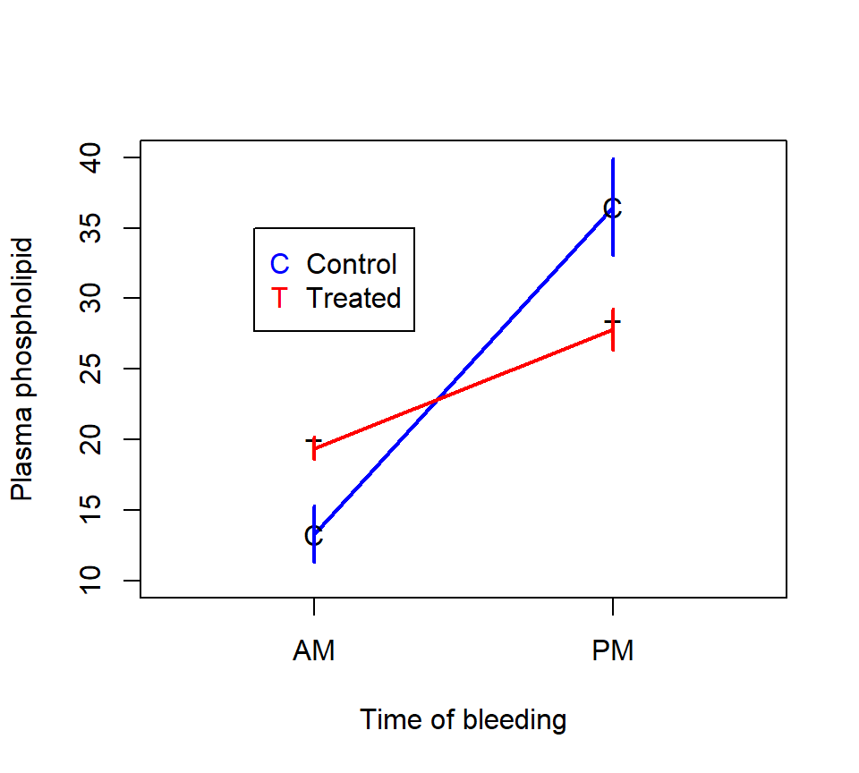
Wilkinson (1954) reports the results of an experiment to study the influence of time of bleeding and diethylstilbestrol (an estrogenic compound) on plasma phospholipid in lambs. Five lambs were assigned at random to each of four treatment groups; treatment combinations are for morning and afternoon bleeding and with and without diethylstilbestrol treatment.
An interaction plot of the data is shown below.
Here is the output of a two-factor ANOVA model using PROC GLM:
proc glm data=sheep;
  class time drug trt;
  model y = time|drug;
run;

                                        Sum of
Source                      DF         Squares     Mean Square    F Value    Pr > F
Model                        3     1539.406600      513.135533      21.61    <.0001
Error                       16      379.923280       23.745205
Corrected Total             19     1919.329880

Source                      DF     Type III SS     Mean Square    F Value    Pr > F
time                         1     1256.746580     1256.746580      52.93    <.0001
drug                         1        8.712000        8.712000       0.37    0.5532
time*drug                    1      273.948020      273.948020      11.54    0.0037
In contrast to the rat example, the interaction here is statistically significant. Because the interaction is significant, the \(F\)-tests of the main effects may no longer have a clear interpretation. Instead, we’ll analyze the simple effects of the two factors. In this case, because each factor only involves two levels, the simple effects can be captured simple (e.g., single df) contrasts. With simple contrasts, it is often more informative to compute an estimate of the contrast instead of merely testing it. The PROC GLM code below uses ESTIMATE statements to compute an estimate of the simple contrast associated with each simple effect:
proc glm data=sheep;
  class time drug trt;
  model y = time|drug;
  estimate 'Simple effect of time, drug=no' time 1 -1 time*drug 1 0 -1 0;
  estimate 'Simple effect of time, drug=yes' time 1 -1 time*drug 0 1 0 -1;
  estimate 'Simple effect of drug, time=AM' drug -1 1 time*drug -1 1 0 0;
  estimate 'Simple effect of drug, time=PM' drug -1 1 time*drug 0 0 -1 1;
run;

Parameter                              Estimate           Error    t Value    Pr > |t|
Simple effect of time, drug=no      -23.2560000      3.08189585      -7.55      <.0001
Simple effect of time, drug=yes      -8.4520000      3.08189585      -2.74      0.0145
Simple effect of drug, time=AM        6.0820000      3.08189585       1.97      0.0660
Simple effect of drug, time=PM       -8.7220000      3.08189585      -2.83      0.0121
Here is a partial interpretation of these contrasts. Sheep with blood drawn in the afternoon have more plasma phospholipid than sheep with blood drawn in the morning, regardless of whether the sheep were given the drug. However, the magnitude of the effect of timing is smaller on sheep given the drug (estimated effect = 8.5 units, s.e. = 3.1) than it is on sheep not given the drug (estimated effect = 23.3 units, s.e.=3.1). For sheep with blood drawn in the afternoon, the drug decreases plasma phospholipid relative to the control (estimated effect = 8.7 units less with the drug, s.e. = 3.1). For sheep with blood drawn in the morning, there is only weak evidence that the drug has an effect on plasma phospholipid (estimated effect = 6.1 units more with the drug, s.e. = 3.1, \(p=0.066\)).
7.2.5 The effects model for a two-factor ANOVA
Just as with one-factor ANOVA, there is an alternative parameterization of the two-factor ANOVA model that uses so-called effects parameters. This parameterization is a bit more useful with the two-factor ANOVA than it was with the one-factor ANOVA.
The effects-model parameterization of the two-factor ANOVA re-expresses each cell mean as the sum of a collection of effects: \[ \mu_{ij} =\mu +\alpha_i +\beta_j +\left(\alpha \beta \right)_{ij} \] Here, \(\mu\) is the reference level, \(\alpha_i\) is the “effect” of level \(i\) of factor A, \(\beta_j\) is the “effect” of level \(j\) of factor B, and \(\left(\alpha \beta \right)_{ij}\) is the interaction between level \(i\) of factor A and level \(j\) of factor B. In one-factor ANOVA, we saw that it was not possible to estimate all the \(\alpha_i\)’s uniquely, so we had to impose a constraint. A similar phenomenon prevails in the two-factor model. How many constraints do we need? The key equivalence is that the number of effects parameters that we can estimate is equal to the number of df for each effect in the df accounting. Thus, while the effects model includes \(a\) different \(\alpha_i\) parameters, we can only estimate \(a-1\) of these parameters uniquely, and thus we require a single constraint. For the interaction parameters, the effects model includes \(a \times b\) different parameters, but we only have \((a-1) \times (b-1)\) df available for the interaction, so we need \(ab - (a-1)(b-1) = a + b -1\) constraints.
Perhaps the most common choice of constraints is the set-to-zero constraint, in which some of the effects parameters are forced to equal zero. Just as with one-factor ANOVA, the set-to-zero constraints are tantamount to building indicator variables in a regression analysis (the effects parameter associated with the baseline, or reference, level is the parameter set to 0).
One advantage to the effects model is that it makes it easier to write down the null hypotheses associated with the ANOVA \(F\)-tests. The ANOVA \(F\)-test associated with comparison of the marginal means of factor A writes as \[ H_0: \alpha_1 = \alpha_2 = \ldots = \alpha_a = 0. \] Similarly, the ANOVA \(F\)-test associated with comparison of the marginal means of factor A writes as \[ H_0: \beta_1 = \beta_2 = \ldots = \beta_b = 0. \] Finally, the ANOVA \(F\)-test associated with the interaction writes as \[ H_0: (\alpha \beta)_{11} = (\alpha \beta)_{12} = \ldots = (\alpha \beta)_{ab} = 0. \] The effects-model parameterization will have additional uses moving forward, for example, when we consider unreplicated or blocked designs.
7.3 Unreplicated factorial designs
Consider an experiment with 5 levels of factor A, 3 levels of factor B, and a single observation for each treatment combination. This is called an unreplicated design because there is only a single replicate for each treatment combination. Let’s try a df accounting for a model that includes main effects of both factors and an interaction:| source | df |
|---|---|
| Factor A | 4 |
| Factor B | 2 |
| A*B interaction | 8 |
| Error | 0 |
| Total | 14 |
This model has no df remaining to estimate the experimental error. Consequently, we cannot estimate \(MS_{Error}\) and hence we cannot conduct \(F\)-tests of the treatment effects.
One option with unreplicated designs is to assume that there is no interaction between the two experimental factors. A model without an interaction is called an additive model. In effects notation, the model is: \[ y_{ijk} =\mu +\alpha_i +\beta_j +\varepsilon _{ijk} \] With an additive model, we use the df that had been allocated to the interaction to estimate the experimental error instead:| source | df |
|---|---|
| Factor A | 4 |
| Factor B | 2 |
| Error | 8 |
| Total | 14 |
The additive model can be used to test for effects of factors A and B. Obviously, these tests are only trustworthy if the assumption of no interactions is appropriate. In biology, it is usually risky to assume that there are no interactions between experimental factors. Additive models for unreplicated designs are more common in industrial statistics.
John Tukey developed a test for additivity with unreplicated factorial designs, sometimes called Tukey’s single degree-of-freedom test. We will not cover Tukey’s test in ST512, although you may want to read about it on your own if you need to analyze an unreplicated factorial design in your own research.
7.4 More than two factors
All of these ideas can be extended to factorial experiments with more than two factors.
Example (based off of an example in Rao (1998)): An investigator is interested in understanding the effects of water temperature (cold vs. lukewarm vs. warm), light (low vs. high), and water movement (still vs. flowing) on weight gain in fish. She has 24 aquaria to serve as experimental units. Each of the 3 x 2 x 2 = 12 treatment combinations are randomly assigned to 2 of the 24 aqauria, and the average weight gain of the fish in each aquaria is measured. This is a balanced three-way factorial design with a CRD randomization structure.
As a first attempt to get a handle on these data, let’s make three different interaction plots, one for each water temperature:
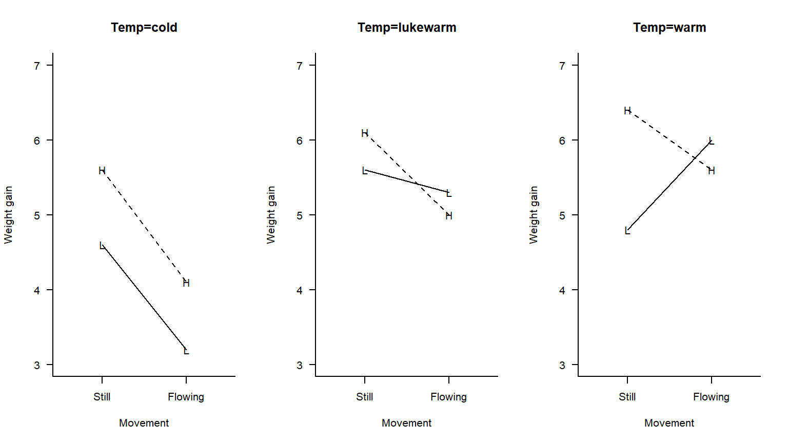 The interaction plot suggests that for some water temperatures, there is an interaction between light levels and water movement. Thus, the way in which the effect of light depends on water movement depends in turn on temperature. Yikes! This is a three-factor interaction. We need a test to see if this interaction is statistically significant, or if it can be attributed to experimental error.
To develop notation for the three-factor model, we’ll extend our ideas from two factor models. For example, \(\mu_{ijk}\) will denote the unknown population mean for the combination of level \(i\) of factor A, level \(j\) of factor B, and level \(k\) of factor C.
With three factors, there are two possible types of interactions:
First-order interactions}: Interactions between two factors
Second-order interactions}: Interactions between first-order interactions
For example, in this experiment the first-order interaction between light level and water movement might describes how the effect of light depends on water movement and vice versa. The second-order interaction describes how this first order interaction may in turn depend on water temperature.
Note that the rules for determining the df associated with higher-order interactions are the same as for first-order interactions: the df are always equal to the product of the df associated with each constituent factor. (Think of this in terms of regression with indicator variables again.)
In effects notation, we can write the cell means as \[ \mu_{ijkl} =\mu +\alpha_i +\beta_j +\gamma _{k} +\left(\alpha \beta \right)_{ij} +\left(\alpha \gamma \right)_{ik} +\left(\beta \gamma \right)_{jk} +\left(\alpha \beta \gamma \right)_{ijk} \] Here, the parameters denoted by \(\left(\alpha \beta \gamma \right)_{ijk}\) capture the second-order interaction among the three factors.
proc glm data=fishgrowth;
  class light temp movement;
  model gain = light|temp|movement;
run;

Example of 3x2x2 factorial from Rao                                                      2
Dependent Variable: gain

                                        Sum of
Source                      DF         Squares     Mean Square    F Value    Pr > F
Model                       11     17.94458333      1.63132576       5.60    0.0030
Error                       12      3.49500000      0.29125000
Corrected Total             23     21.43958333

Source                      DF     Type III SS     Mean Square    F Value    Pr > F
light                        1      2.10041667      2.10041667       7.21    0.0198
temp                         2      7.64333333      3.82166667      13.12    0.0010
light*temp                   2      0.64333333      0.32166667       1.10    0.3629
movement                     1      2.47041667      2.47041667       8.48    0.0130
light*movement               1      1.35375000      1.35375000       4.65    0.0521
temp*movement                2      2.89333333      1.44666667       4.97    0.0268
light*temp*movement          2      0.84000000      0.42000000       1.44    0.2746
The analysis strategy with a three-way factorial design is similar to the analysis strategy with a two-way factorial design:
Test for the significance of the second-order interaction.
If the second-order interaction is significant, either unpack the factorial treatment structure and treat the design a one-factor ANOVA, or ``divide and conquer’’ by analyzing the effects of two factors at each level of the third factor.
If the second-order interaction is not significant, you may remove the second-order interaction and re-fit the model, although this is not necessary. Test for the significance of the first-order interactions. If any of the first-order interactions are significant, analyze simple effects. If none of the first-order interactions are significant, analyze main effects.
In the example above, the second-order interaction is not statistically significant (\(F_{2, 12} = 1.44\), \(p = 0.27\)). The only statistically significant first-order interaction is the interaction between water temperature and movement (\(F_{2,12} = 4.97\), \(p = 0.027\)). Neither of the first-order interactions involving light are statistically significant (although the light-by-movement interaction is on the border of statistical significance, \(F_{1,12} = 4.65\), \(p = 0.052\)). The main effect of light is statistically significant (\(F_{1,12} = 7.21\), \(p = 0.020\)). We could then proceed by quantifying the main effect of light with a linear combination, and quantifying the simple effects of movement at different water temperatures.
Main effect of light: \[\theta _{light} =\bar{\mu}_{1++} -\bar{\mu}_{2++} \] Simple effect of movement when temperature = cold: \[\theta _{m/C} =\bar{\mu}_{+11} -\bar{\mu}_{+12} \] Simple effect of movement when temperature = lukewarm: \[\theta _{m/L} =\bar{\mu}_{+21} -\bar{\mu}_{+22} \] Simple effect of movement when temperature = warm: \[\theta _{m/W} =\bar{\mu}_{+31} -\bar{\mu}_{+32} \]
A final note: unreplicated three-way factorial designs are not uncommon in the life sciences. To analyze these designs, one typically assumes that there is no second-order interaction, and uses the df that would have been absorbed by the second-order interaction as the df for error. Some will argue that higher-order interactions are rare in nature, and thus assuming that they do not occur is justified. Whether you agree with this or view it as a just-so rationalization is up to you.
7.5 Analysis using PROC GLM in SAS
Consider the following example taken from Sokal and Rohlf (1995). This experiment was designed to examine differences in food consumption among rats. 6 male rats and 6 female rats were used in the experiment. Half the rats were fed fresh lard (fat), and half the rats were fed rancid fat. The response is total food consumption (in grams) over 73 days. This is a 2 \(\times\) 2 factorial design with a CRD. The experiment is balanced.
To use PROC GLM to compute the two-factor ANOVA table, we would use
proc glm data=rat;
  class trt sex fat;
  model food = sex fat sex*fat;
run;
The ANOVA \(F\)-tests are contained in the output:
                                        Sum of
Source                      DF         Squares     Mean Square    F Value    Pr > F
Model                        3     65903.58333     21967.86111      15.06    0.0012
Error                        8     11666.66667      1458.33333
Corrected Total             11     77570.25000

Source                      DF     Type III SS     Mean Square    F Value    Pr > F
sex                          1      3780.75000      3780.75000       2.59    0.1460
fat                          1     61204.08333     61204.08333      41.97    0.0002
sex*fat                      1       918.75000       918.75000       0.63    0.4503
The first portion of the output above gives the sum-of-squares breakdown and associated ANOVA \(F\)-test if we were just treating the data as a one-factor ANOVA. That is, the \(F\)-test in the first table is a test of \(H_0\): \(\mu_{11} =\mu_{12} =\mu_{21} =...=\mu_{ab}\). (This is equivalent to a model-utility test in multiple regression.) The second portion of the output provides \(F\)-tests for the main and interaction effects.
PROC GLM also provides two sum-of-squares decompositions, one which it calls Type I and another which it calls Type III. Type I and Type III sum-of-squares are identical for balanced factorial designs. They are not identical for unbalanced designs. We will discuss the differences for unbalanced designs later.
In the model statement, we can use a vertical bar as shorthand for including both main effects and interactions. The code below would produce identical output to the code above:
proc glm data=rat;
  class trt sex fat;
  model food = sex|fat;
run;
PROC GLM uses set-to-zero constraints. We can see the constraints by calling for SAS’s parameter estimates with the SOLUTION option to the MODEL statement in PROC GLM:
proc glm data=rat;
  class trt sex fat;
  model food = sex|fat / solution;
run;

The GLM Procedure
                                                  Standard
Parameter                       Estimate             Error    t Value    Pr > |t|
Intercept                    535.3333333 B     22.04792759      24.28      <.0001
sex       female             -18.0000000 B     31.18047822      -0.58      0.5796
sex       male                 0.0000000 B       .                .         .
fat       fresh              160.3333333 B     31.18047822       5.14      0.0009
fat       rancid               0.0000000 B       .                .         .
sex*fat   female fresh       -35.0000000 B     44.09585518      -0.79      0.4503
sex*fat   female rancid        0.0000000 B       .                .         .
sex*fat   male fresh           0.0000000 B       .                .         .
sex*fat   male rancid          0.0000000 B       .                .         .

NOTE: The X'X matrix has been found to be singular, and a generalized inverse was used to
solve the normal equations.  Terms whose estimates are followed by the letter 'B'
are not uniquely estimable.
Now, to calculate the main effect of fat using SAS, we have to recode our linear combination in terms of the parameters in the effects model. Here goes: \[\begin{eqnarray*} \theta _{fat} & = & \frac{1}{2} \left(\mu_{12} +\mu_{22} -\mu_{11} -\mu_{21} \right) \\ & = & \frac{1}{2} \left(\mu +\alpha _{1} +\beta _{2} +\left(\alpha \beta \right)_{12} +\mu +\alpha _{2} +\beta _{2} +\left(\alpha \beta \right)_{22} -\mu -\alpha _{1} -\beta _{1} -\left(\alpha \beta \right)_{11} -\mu -\alpha _{2} -\beta _{1} -\left(\alpha \beta \right)_{21} \right) \\ & = & \frac{1}{2} \left(2\beta _{2} +\left(\alpha \beta \right)_{12} +\left(\alpha \beta \right)_{22} -2\beta _{1} -\left(\alpha \beta \right)_{11} -\left(\alpha \beta \right)_{21} \right) \\ & = & -\beta _{1} +\beta _{2} -\frac{1}{2} \left(\alpha \beta \right)_{11} +\frac{1}{2} \left(\alpha \beta \right)_{12} -\frac{1}{2} \left(\alpha \beta \right)_{21} +\frac{1}{2} \left(\alpha \beta \right)_{22} \end{eqnarray*}\] Now we can read off the coefficients from the last line of the expression above and feed them into an ESTIMATE statement. Note that this combination only involves parameters for the ‘fat’ effect and the interaction:
proc glm data=rat;
  class trt sex fat;
  model food = sex|fat;
  estimate 'Fresh v. rancid' fat -1 1 sex*fat -.5 .5 -.5 .5;
run;

Parameter                   Estimate  Standard Error    t Value    Pr > |t|
Fresh v. rancid          -142.833333      22.0479276      -6.48      0.0002
As always, SAS provides (for free) a \(p\)-value for the test of \(H_0\): \(\theta =0\) vs. \(H_a\): \(\theta \ne 0\). For illustration’s sake, we can also write linear combinations for the main effect of sex, and for the interaction effect. One way to write these linear combinations is: \[\theta _{sex} =\frac{\mu_{21} +\mu_{22} }{2} -\frac{\mu_{11} +\mu_{12} }{2} \] and \[\theta _{int} =\left(\mu_{22} -\mu_{12} \right)-\left(\mu_{21} -\mu_{11} \right)\] Using PROC GLM, we estimate these effects as
proc glm data=rat;
  class trt sex fat;
  model food = trt;
  estimate 'Fresh v. rancid' fat -1 1 sex*fat -.5 .5 -.5 .5;
  estimate 'Male v. female'  sex -1 1 sex*fat -.5 -.5 .5 .5;
  estimate 'Interaction'     sex*fat 1 -1 -1 1;
run;

Parameter                   Estimate  Standard Error    t Value    Pr > |t|
Fresh v. rancid          -142.833333      22.0479276      -6.48      0.0002
Male v. female            -35.500000      22.0479276      -1.61      0.1460
Interaction                35.000000      44.0958552       0.79      0.4503
Thus, to summarize our analysis of this experiment: There is no evidence of a statistically significant sex effect. There is strong evidence of an effect of fat on food consumption (\(F_{1,8} = 41.97\), \(p=0.0002\)). Rats fed rancid fat consumed on average 142.9g (s.e. 22.0g) less food than rats fed fresh fat.